-
-
Course Introduction
-
Two Kinds of Paths
-
Polynomials vs. Exponentials
-
Divide and Conquer
-
Big O and All that
-
When the details don't matter
-
Quiz 1 (self-assessment)
-
-
-
Divide and Conquer Redux
-
Dynamic Programming
-
Greedy Algorithms
-
Landscapes
-
Reductions and Translations
-
Lessons So Far
-
The Best of All Possible Algorithms
-
Complexity Wrap-Up
-
Quiz 2 (self-assessment)
-
-
-
Finding versus Checking
-
Circuits and Formulas
-
More NP-complete Problems
-
P versus NP Problem
-
Existence and Nonexistence
-
Above and Beyond
-
Quiz 3 (self-assessment)
-
-
-
Real World Problems
-
Phase Transitions
-
Random Problems
-
Solvability Threshold
-
Modeling Differential Equations
-
Landscapes, Clustering, Freezing, and Hardness
-
Quiz 4 (self-assessment)
-
-
-
Building Blocks: Recursive Functions
-
Building Blocks: Partial Recursive Functions
-
λ Calculus
-
Turing Machines
-
The Halting Problem
-
The Grand Unified Theory of Computation
-
The Analytical Engine
-
Cellular Automata
-
Tile-Based Computation
-
Dynamical Systems
-
Quiz 5 (self-assessment)
-
-
-
More from Cris Moore
-
Other ComplexityExplorer resources
-
1.7 Quiz 1 (self-assessment) » Quiz 1: Explanation
Q1. What does it mean to “compute” in a way that many complex systems “compute”?
(A) To perform a mathematical calculation.
(B) To store, transmit, and transform information.
(C) To use an algorithm to arrive at an output from given inputs.
(D) To simulate a world/system in a predictive way.
Explanation: Besides Cris’s quote in lecture 1.2 (0:15, “information is being stored, transmitted, and transformed - that’s what computation is”), the definition of complex systems is inherently based in information and information theory. Claude Shannon’s formation of information theory (summarized here by SFI's Simon DeDeo, 2018) has provided the means of analyzing complex systems, and is frequently used in measures of complexity (Lloyd, 2001). Complex systems can perform mathematical calculations, use algorithms, or simulate a world/system, but the actual computation is rooted in information.
Q2. Why is it preferable to find a solution to a problem that takes polynomial rather than exponential time?
(A) A polynomial-time solution means the problem is easy.
(B) A polynomial-time solution always takes less computational time.
(C) A polynomial-time solution indicates that the problem is understood in a general, coarse-grained sense.
(D) All of the above.
Explanation: A polynomial-time problem is in the form O(nc), where n is the size of the input and c is a constant. This form puts a specific constraint on the number of times (c) an algorithm iterates over the input. For example, if c = 3, then the algorithm at worst iterates through the input 3 times. This implies a general understanding of the problem at hand.
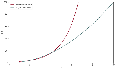
This does not mean the problem is easy. Apart from the fundamental question of “what is easy?”, c can be an arbitrarily large number, thus making a problem computationally intractable. Additionally, for certain low values of n and c, exponential time is faster (see graph below). However, as n and c approach infinity, exponential time grows much quicker than polynomial (see figure below, with c=2).

Q3. What differs between an Eulerian path and a Hamiltonian path through a graph?
(A) Eulerian paths traverse all edges. Hamiltonian paths visit all nodes.
(B) Eulerian paths can be found in polynomial time. Hamiltonian paths are found in exponential time.
(C) The existence of an Eulerian path can be computed without exhaustive search. Hamiltonian paths must be found through exhaustive search.
(D) All of the above.
Explanation: There are many sources which explain the difference between Eulerian and Hamiltonian paths, including this class in lecture 1.2. Here are a few: Greg Baker’s Discrete Math course notes at Simon Fraser University CS; the Wikipedia page of Hamiltonian paths, which gives more historical information not covered in this class; and a real-world application of Eulerian and Hamiltonian paths in autonomous surface vehicles (Arzamendia et al, 2017).
Q4. Which of the following is usually the limiting resource - i.e. that which we need to minimize - in a computer program?
(A) Energy.
(B) Communication.
(C) Memory.
(D) Time.
(E) Hardware.
Explanation: Modern computing is so powerful, constraints which were once problems are no longer issues. Supercomputers have access to petabytes of memory and perform massively parallel computation across wide distances, while hardware continuously improves, even if Moore’s Law is running into atomic limitations (Hesseldahl, 2016). Computational energy - while part of a larger conversation regarding energy infrastructure (Jones, 2018) - is fairly cheap and readily accessible. Computational time, which is defined here as the number of computational operations needed to perform a task, hasn’t changed much over time, and therefore is usually the limiting factor for a program.
Q5. You have written a program S that solves problem Q in 7 seconds for an input size s=5 (O(s2)). You have written another program R that solves problem Q in 3.5 seconds for an input size s=5 (O(s log s)). Now you need to find the solution for an input size s=500. Would you prefer to run program Q or program R with s=500, assuming that you want the solution as fast as possible?
Q5 (A): Based on the Big O of program S, O( s^2 ), how many calculations does program S perform for an input size of 5 in the worst case?
(A) 1
(B) 5
(C) 10
(D) 25
Explanation: Since the input is 5 and in the worst case, the number of steps is s^2, there are 25 computational steps in Program S.
Q5 (B): Based on the Big O of program R, O( s * log(s) ), how many calculations does program R perform for an input size of 5 in the worst case?
(A) 3.5
(B) 5
(C) 5.5
(D) 10
Explanation: For an input of 5 and a worst case of s*log(s), there are 5*log(5) computational steps, which simplifies to 5*0.70 and further to 3.5 computational steps.
Q5 (C): Based on your answer in part (a), at what speed (in calculations per second) does program S run in the worst case?
(A) 1.68
(B) 3.57
(C) 7.14
(D) 10.0
Explanation: Since there are 25 computational steps in Program S and it runs in 7 seconds, each second holds 25 / 7 computational steps, or 3.57 steps per second.
Q5 (D): Based on your answer in part (b), at what speed (calculations per second) does program R run in the worst case?
(A) 1
(B) 3
(C) 10
(D) 15
Explanation: Similar to 5(C), since there are 3.5 computational steps in Program R and it runs in 3.5 seconds, each second holds 3.5/3.5 computational steps, or 1 step per second.
Q5 (E): What program (S or R) would you prefer to run for an input size of 50000, and why?
(A) Program S, it is significantly faster than Program R
(B) Program S, it is slightly faster than Program R
(C) Program R, it is significantly faster than Program S
(D) Program R, it is slightly faster than Program S
(E) Either - they are equivalent
Explanation: This question has a few layers. The first is that O(n log n) is much more computationally efficient than O(n2). For n = 5, Program R only needs to do 3.5 calculations, while Program S has to do 25 calculations. The pattern found in parts (C) and (D) hold as n increases, with the number of calculations required to do Program S increasing much faster than Program R. At n = 500, Program S does 250000 steps (5002), while Program R does only 1349.48 steps (500 * log(500) ). See the figure below for a visual representation of this difference and how quickly program S increases in comparison to program R (the y-axis represents steps).
Another way of looking at this problem is to calculate the time per calculation step: maybe the computation in Program S (3.57 computational steps per second) is quick enough to overcome the vast difference in number of steps? However, as the table below shows, Program R (1 computational step per second) still finishes ~700 times faster.


Q6. What is the factor of n that determines BigO for the following functions?

(A) A = O(n4) B = O(n2) C = O(2n2)
(B) A = O(n3) B = O(n) C = O(n3 log n)
(C) A = O(n5) B = O(n2) C = O(n log n)
(D) A = O(n3) B = O(n2) C = O(n2)
Explanation: This is explained in detail in lecture 1.5. By definition, BigO refers to the limiting behavior of a function as the function tends toward infinity. As a function grows toward infinity, the quickest-growing term becomes the limiting factor. In this case, n^x is the fastest growing term in each function, with larger x’s growing faster. Additionally, all constants are ignored. For a hierarchy of BigO complexities outside of this question, here’s an easy cheat sheet (Rowell, 2016).
Q7. What is the immediate next step in this divide-and-conquer algorithm for multiplication?

(A) Repeat the algorithm on 12, 98, 34 and 76..
(B) Complete the calculation shown on the bottom line.
(C) Calculate X1, X2 and X3, as indicated.
(D) None of the above.
Explanation: This divide-and-conquer multiplication algorithm, also known as the Karatsuba algorithm, assumes that the most simple form of multiplication is between two one-digit numbers and a power of 10. That is, instead of 13*2, it would be preferable to calculate (1*2) * 101 + (3*2) * 100. Since none of the given options express this form, it is necessary to recursively continue the algorithm on 12, 98, 34, and 76 in order to further simplify the problem.
Q8. In the pseudocode below, identify the BigO category for the two steps - A and B - indicated. A refers to the "for" statement; B refers to the "print" statement.

(A) A = linear; B = linear
(B) A = logarithmic; B = constant
(C) A = logarithmic; B = linear
(D) A = linear; B = constant
Explanation: In simple terms, BigO refers to how the number of computational steps in an algorithm grows as the number of items increases. For the for loop in part A, as the data variable grows, the number of steps will increase linearly: append() is a one-step method where x is added to the end of the data_0 list. In this case, there are 4 computational steps - if data held 10 numbers, there would be 10 computational steps. In part B, look-up in a list in python is a one-step process, regardless of how long the list is. Therefore, it is a constant BigO.
Note: For those interested, here is a list of the BigO of various python list operations.
Q9. Is there an Eulerian path through the graph below? Why or why not?

(A) Yes, there are three or fewer nodes that have odd numbers of connections (edges).
(B) Yes, through a brute-force search, one can find a path through all nodes.
(C) No, there are an even number of nodes and an even number of connections (edges).
(D) No, there are more than two nodes that have odd numbers of connections (edges).
Explanation: In order for an Eulerian path to exist, there must be a unique starting and ending point, and these nodes must be the only nodes with an odd number of edges. Otherwise, one or more of those odd-numbered edges will be left untraveled, since there is no way to return to that particular node once it is already visited and satisfy the conditions of Eulerian path. As this graph has four nodes with an odd number of edges, it does not satisfy the conditions for an Eulerian path.
Note: For further reading on Eulerian paths (and graph theory in general), check out Chapter 2 of Albert Barabasi’s free textbook on network science (Barabasi, 2013).
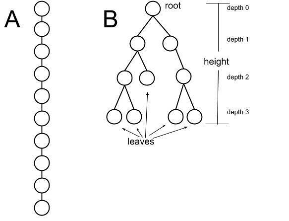
Q10. The diagram below illustrates linear (A) and binary tree (B) data structures, containing identical data. Each entry in the data structures is a name. You develop algorithms that take a query name and search the data structures to see if that name exists in the entries. The entries are not sorted. The following questions apply to these data structures and the corresponding search algorithms.

Q10 (A): On average, which performs the search faster?
(A) Linear (A)
(B) Binary tree (B)
(C) Both are the same
Explanation: Since both data structures are unsorted, it is unknown where the query exists and therefore, a search over both structures will (at worst) search every node in the data structure. Therefore, both structures search in O(n) time.
Q10 (B): Assuming that the query names are random, what should be the first step after checking the root node in the binary tree search (B)?
(A) Check the child node on the left branch.
(B) Check the child node on the right branch.
(C) Randomly check the child node on either the left or right branch.
(D) Any of the above.
Explanation: The binary tree structure is only useful for search with sorted lists (see parts c & f). In the random case, every node needs to be checked regardless of placement in the tree, so it does not matter in which order the search is performed. There is no cost associated with backtracking or jumping around in a data structure (see Q8 for the BigO of accessing an item in a list).
Q10 (C): Would the binary tree search (B) be more or less efficient, or the same, if: the names in the data structure were alphabetized; and the search branch was chosen according to alphabetical relationship of the query name?
(A) More efficient ~ faster
(B) Less efficient ~ slower
(C) Same efficiency ~ same speed
Explanation: Using alphabetized lists will allow the algorithm to decide on a direction at each branch, thereby ignoring half of the existing tree at each step. This dramatically reduces the number of computational steps needed from n to log(n), which makes this sorted binary tree much more efficient, and therefore faster.
Note: For an interesting visualization of binary search trees, check out this tool from the University of San Francisco (note: works best on Chrome).
Q10 (D): Could the linear search (A) be more or less efficient, or the same, if: the data structure were "circular"; the search started in a random location each time; and the search direction was chosen randomly?
(A) More efficient ~ faster
(B) Less efficient ~ slower
(C) Same efficiency ~ same speed
Explanation: A circular data structure may be useful (see part (e)), but since the starting point and direction are chosen randomly, no efficiency is gained. As with the initial linear structure, the worst case scenario is that every node is visited.
Q10 (E): Would the linear search (A) be more or less efficient, or the same, if: the data structure were "circular"; the search started in a random location each time; the data structure were alphabetized; and the search direction was chosen according to alphabetical relationship of the query name?
(A) More efficient ~ faster
(B) Less efficient ~ slower
(C) Same efficiency ~ same speed
Explanation: The addition of sorting and choosing direction by sorted relationship to the query causes this method to be more computationally efficient. In the worst case, the search will travel n/2 nodes (see image below). While the BigO does not change, the functional speed does change and will result in a more efficient, faster algorithm.
In general, BigO is a powerful way to analyze the performance of your algorithm. However, if you are writing code designed for performance, BigO can only get so far - there are other tricks that you can utilize to ensure your code is running as fast as possible.

Q10 (F): If two more entries (nodes) were added to the sorted binary tree (B) below the leaf at depth 2, would the efficiency of the search change?
(A) No, the speed is determined by the height of the tree.
(B) Yes, more nodes require more time to traverse.
(C) No, as long as the algorithm searches the left branch first.
(D) Yes, the speed is determined by the number of leaves.
Explanation: In the original sorted binary tree, the maximum number of computational steps needed in the worst case is 3 (depth). If two nodes are added at depth 3, this maximum number of steps does not change. The BigO remains the same – O(log n) – and so does the functional speed.

